Tutorial#
Basic usage and error estimation#
In this tutorial, we explain the basic usage of dacp to compute eigenvalues of sparse matrices – including degeneracies.
We also show the algorithm’s precision and how to estimate errors.
Show code cell source
from dacp.solver import estimated_errors, eigvalsh
import matplotlib.pyplot as plt
from matplotlib import rc
import numpy as np
from scipy.sparse import diags, eye
from scipy.sparse import kron
Let us start computing the eigenvalues of a random tri-diagonal hermitian matrix. For comparison, we perform dense diagonalization.
# Set matrix size (N x N)
N = int(5e2)
# Set main diagonal
b = 2 * (np.random.rand(N) - 0.5)
# Set
c = 2 * (np.random.rand(N - 1) + np.random.rand(N - 1) * 1j - 0.5 * (1 + 1j))
# Create matrix
H = diags(c, offsets=-1) + diags(b, offsets=0) + diags(c.conj(), offsets=1)
# Perform dense diagonalization
true_vals = np.linalg.eigvalsh(H.todense())
We now run the DACP eigenvalue solver. We pass the matrix itself and set a window within the computed eigenvalues will be in.
window = [-0.1, 0.2]
evals = eigvalsh(H, window=window)
We now compare the eigenvalues computed via dense diagonalization and DACP and compute the relative error.
Show code cell source
map_eigv = []
for value in evals:
    closest = np.abs(true_vals - value).min()
    map_eigv.append(true_vals[np.abs(true_vals - value) == closest][0])
true_vals = np.array(map_eigv)

fig, axs = plt.subplots(1, 2, figsize=(10, 4))

true_vals = np.sort(true_vals)
n = np.arange(-evals.shape[0] / 2, evals.shape[0] / 2)
axs[0].scatter(n, evals, c="k", label="DACP")
n_true = np.arange(-true_vals.shape[0] / 2, true_vals.shape[0] / 2)
axs[0].scatter(n_true, true_vals, c="r", s=4, label="dense diag.")
axs[0].set_ylabel(r"$\lambda_i$")
axs[0].set_xlabel(r"$n$")
axs[0].set_title('Eigenvalues')
axs[0].legend()

axs[1].scatter(evals, np.abs((true_vals - evals) / true_vals))
axs[1].set_ylabel(r"$|\delta \lambda_i / \lambda_i|$")
axs[1].set_xlabel(r"$\lambda_i$")
axs[1].set_yscale("log")
axs[1].set_title("Relative error")

plt.tight_layout()
plt.show()
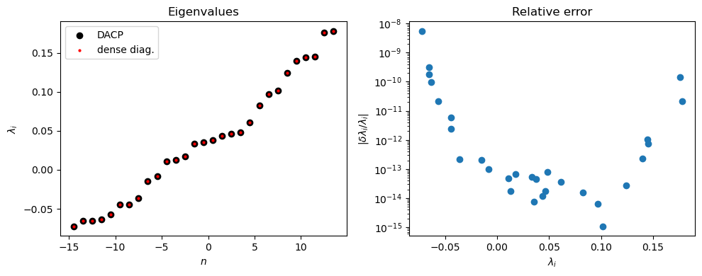
The errors are larger at the edges of the desired window because the quality of the filter decreases. Because the errors are deterministic, our interface also provides an estimation of the relative error (red line) that we compare with the errors calculated from dense diagonalization (black dots). For better visualization, we also plot a window (red shade) of 1% to 10000% of the estimation.
Ei = np.linspace(window[0], window[1], 300)
eta = estimated_errors(
    Ei,
    window,
)
Show code cell source
plt.plot(Ei, eta, "r", label="estimated error")
plt.fill_between(Ei, 0.01 * eta, 100 * eta, alpha=0.4, fc="r")
plt.scatter(evals, np.abs((true_vals - evals) / evals), c="k", zorder=10, s=1, label="computed error")
plt.ylabel(r"$|\delta \lambda_i/\lambda_i|$")
plt.xlabel(r"$\lambda_i$")
plt.yscale("log")
plt.xlim(window[0], window[1])
plt.legend()
plt.show()

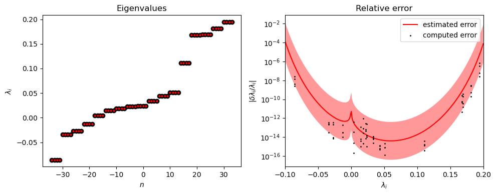
Degenerate spectrum#
The original proposal of DACP suggests solving the eigenvalue problem many times to resolve degeneracies. Our algorithm resolves degeneracies systematically to facilitate usage. To showcase our implementation, we create a random tridiagonal matrix for which all eigenvalues are 4-fold degenerate and again compare with dense diagonalization. We use the same eigenvalue window from the previous part of the tutorial. We observe that the degeneracies are resolved and the precision remains.
N = int(250)
c = 2 * (np.random.rand(N - 1) + np.random.rand(N - 1) * 1j - 0.5 * (1 + 1j))
b = 2 * (np.random.rand(N) - 0.5)

H = diags(c, offsets=-1) + diags(b, offsets=0) + diags(c.conj(), offsets=1)
H = kron(H, eye(4))

true_vals = np.linalg.eigvalsh(H.todense())
evals = eigvalsh(H, window=window)
Show code cell source
map_eigv = []
for value in evals:
    closest = np.abs(true_vals - value).min()
    map_eigv.append(true_vals[np.abs(true_vals - value) == closest][0])
true_vals = np.array(map_eigv)

fig, axs = plt.subplots(1, 2, figsize=(10, 4))

true_vals = np.sort(true_vals)
n = np.arange(-evals.shape[0] / 2, evals.shape[0] / 2)
axs[0].scatter(n, evals, c="k")
n_true = np.arange(-true_vals.shape[0] / 2, true_vals.shape[0] / 2)
axs[0].scatter(n_true, true_vals, c="r", s=4)
axs[0].set_ylabel(r"$\lambda_i$")
axs[0].set_xlabel(r"$n$")
axs[0].set_title("Eigenvalues")

axs[1].plot(Ei, eta, "r", label="estimated error")
axs[1].fill_between(Ei, 0.01 * eta, 100 * eta, alpha=0.4, fc="r")
axs[1].scatter(evals, np.abs((true_vals - evals) / evals), c="k", zorder=10, s=1, label="computed error")
axs[1].set_ylabel(r"$|\delta \lambda_i/\lambda_i|$")
axs[1].set_xlabel(r"$\lambda_i$")
axs[1].set_yscale("log")
axs[1].set_xlim(*window)
axs[1].set_title("Relative error")
axs[1].legend()

plt.tight_layout()
plt.show()